Tupper tests out a statistical approach to similarity

Approaching Imitation Masses Through Melodic Similarity

Laura L. Tupper (Mount Holyoke College)

Introduction

In this paper, we discuss a data-driven perspective on the CRIM project. Using tools for the analysis of quantitative data, with and without additional information about the subject matter, can both support human-expert conclusions and reveal new insights. Here we focus on the concepts of mathematical similarity and distance, and explore how they can be applied to the data at multiple levels. These ideas allow us to compare many different types of objects to one another, from individual notes to entire pieces.

In statistical analysis, we often seek to quantify the similarity between different objects, using a similarity measure (or, equivalently, its opposite: a dissimilarity or distance measure). This process first requires finding a quantitative representation of the objects we are analyzing. For example, we might represent a melodic phrase, a harmonic phrase, a voice line, or an entire piece of music using a series of numbers. Of course, there are many possible representations we could create. A representation might be as simple as “largest interval in this phrase” or “number of voices in this piece,” but could also be more complex in order to reflect more information about the object. Some of these possible representations are described in the following sections.

Once we have this representation of each musical phrase, piece, or other object, we can calculate a numerical similarity or dissimilarity between any pair of objects. At this stage there is also a broad choice of methods, though there are some typical commonalities across methods: for example, the dissimilarity or distance between two identical objects is usually set to be 0, with objects that are more different from each other having a greater distance (and lower similarity).

We can examine these pairwise similarity or distance values directly, or compare them against each other: for example, we might be able to see that a certain Mass movement is more similar to the model than another movement in the same Mass, or that it is more similar to its own model than another motet. Ultimately, we may be able to group objects together into classes or clusters, and explore what musical behaviors correspond to the quantitative commonalities we have found among them.

Quantitative Representations

Intervals and time series

First, we discuss the representation of musical score data as quantitative values. Like many other analysts in the CRIM project, we use an interval representation: we record the musical interval between each consecutive pair of pitches in each voice. Using intervals, rather than fixed pitch values, allows us to convey the melodic shape of a piece while ignoring that piece’s key and any transpositions.

Translating a piece into interval form is the most basic application of distance and similarity concepts to the data, as we are recording the distance between pitches. Even at this level, the choice of distance measure is not trivial. For example, we must choose whether to use a strict count of half-steps or scale degrees (chromatic or diatonic pitch space), whether to count a repeated pitch as an interval of 0 or as no interval at all (merging unisons, a process which can find melodic similarity when a phrase or motif is broken up to account for a different text, as frequently happens during the kinds of adaptation encountered in the Imitation Mass repertory), how to manage octaves, and so on. In our analysis, we use the diatonic pitch space, but shift the interval values from musical to mathematical terms by making a unison equal to 0, an ascending second equal to 1, a descending second equal to -1, and so on.

Each interval has a corresponding time point, which may be represented as consecutive indices (incrementing by one for each new pitch, regardless of the note’s duration) or as a position within the piece (the number of beats since the start of the piece). This allows us to consider any voice or melodic line as a time series, a form of data consisting of an ordered sequence of values with an accompanying time point for each value. For example, we might denote “the interval beginning at beat 12 is a descending second” as $t_{12} = -1$ . If we consider different voices together, we have a multivariate time series, with multiple values associated with each time point. In our analysis, we use offset sampling, measuring the pitch at regular intervals throughout the piece regardless of whether a new note occurs in the score on that beat, then calculating the intervals between these sampled pitches. This approach means that the intervals’ time points are regularly spaced, and consistent across different voices and pieces. The resolution chosen for the offset can determine what musical behaviors are represented. For example, a short offset will sample the piece frequently, reflecting short-term melodic changes and details. A longer offset, such as sampling every four beats, will ignore ornamentation and can help bring out a melodic line’s underlying form, but may miss faster-paced melodic phrases. We choose a medium resolution, sampling every two beats.

Figure 1 shows the interval representation of an example piece, the beginning of Josquin’s Mente Tota from Vultum tuum (CRIM Model 0016). Each point shows the value of an interval as well as its time point. If a voice is resting at a given time point, it has no interval value at that time; this also applies if one side of the interval is a rest, as when a voice enters, since we do not calculate an interval between a fixed pitch and silence.

We can better understand this data representation by comparing part of the score of Mente Tota. At the start of the piece, the Contratenor begins with the motif shown in Figure 2. In the time series plot, this is represented in the “Contratenor” sub-plot as a value of 0 at time 2 (the sustained pitch in the first bar, which is recorded as a unison between the pitches at beat 0 and beat 2); 0 at times 4, 6, 8, and 10; -1 at time 12 (reflecting the descending second between beat 12 and beat 14); 0 at time 14; 1 at time 16; and so on. We can also see this sequence of (0, 0, 0, 0, 0, -1, 0, 1) occur at the beginning of each voice line, as each voice opens with the same motif.

More generally, this type of interval visualization gives a sense of a piece’s motion, rather than its absolute pitches. Areas with long sequences of mostly 0 values show when a voice is moving slowly, with many unisons; areas with many values farther from 0 (for example, the period around time 400 in this figure, in all voices) reflect times of greater melodic motion; and particularly large leaps stand out as very high (or very negative) intervals, as with the leap in the Bassus near time 500.

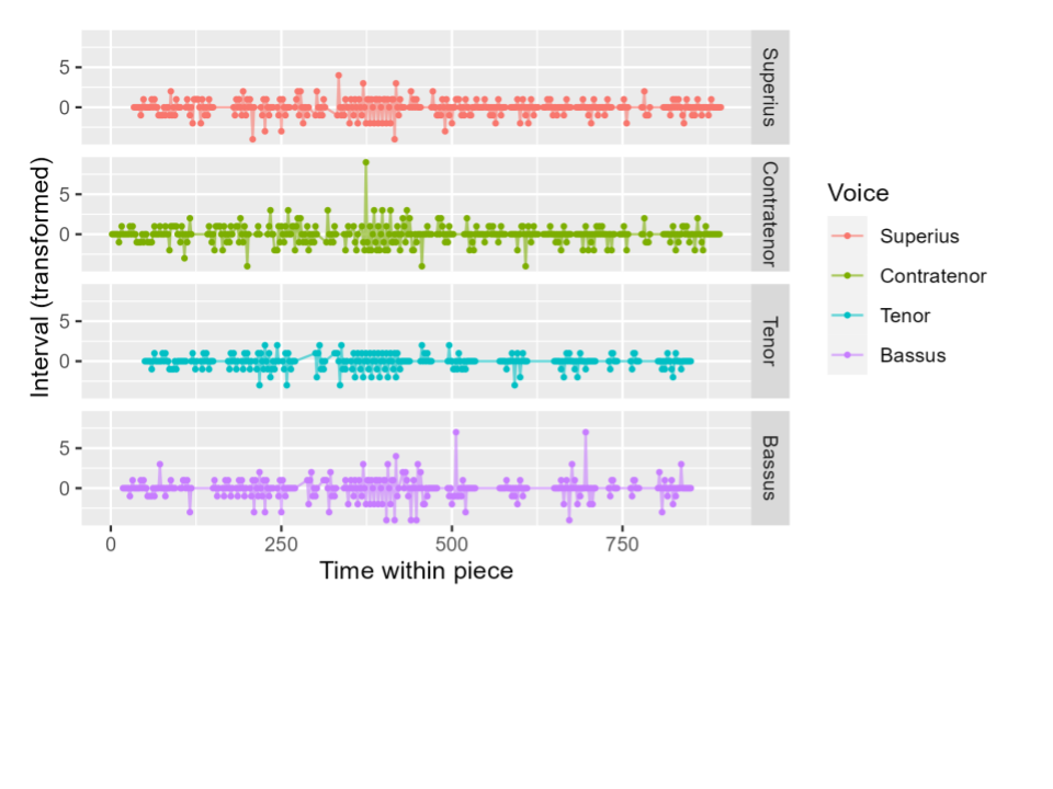
Figure 1. Interval representation of Josquin’s Mente Tota, separated by voice. The x coordinate of each point indicates the time within the piece (number of beats from start), and the y coordinate indicates the size of the interval between the pitch at that time and the following pitch. Intervals are diatonic, but shifted so that a unison is 0.

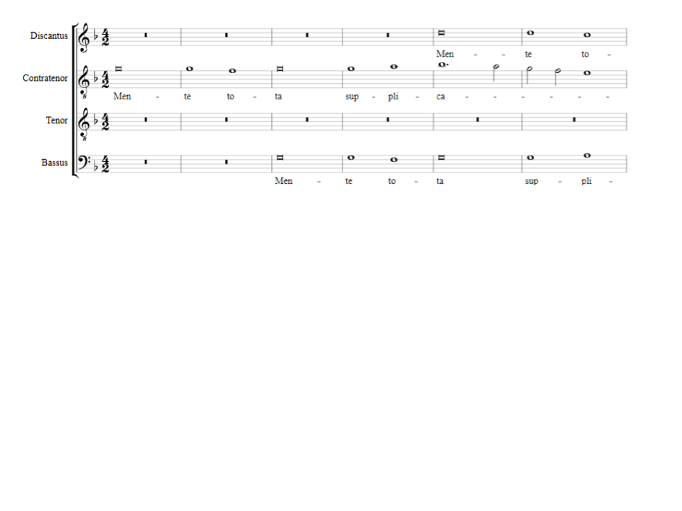
Figure 2. Beginning of the score of Josquin’s ***Mente Tota*. The initial pattern of unisons and seconds in each voice line corresponds to the sequence (0, 0, 0, 0, 0, -1, 0, 1) that begins each line in the interval representation.**

n-grams

Between the individual interval and the time series of an entire piece or melodic line, we can examine an intermediate scale: short sequences of consecutive intervals. We refer to these as n-grams, where n represents the number of intervals included in each sequence. For example, the 5-gram beginning at time 10 of Josquin’s Mente Tota in the Contratenor is (0, −1, 0, 1, 0): a unison, descending second, unison, ascending second, and unison, in that order.

From a data analysis perspective, choosing different n-gram lengths will suggest different analytical tools and reflect different types of musical behavior, though any value of n may lead to interesting results. When n is quite small, such as 1 or 2, the n-grams are very short, and will not necessarily correspond to what a human listener would think of as a melodic phrase. But they can be enumerated, and we can examine a piece’s usage of the different possible n-grams as a kind of melodic vocabulary (see “Frequency distributions” below).

When n is larger, the corresponding n-grams are longer, and there are vastly more sequences that are mathematically possible. It is no longer useful to enumerate all these possibilities: for example, there are over 100 million possible 7-grams (even assuming a constrained range of possible values for any individual interval), most of which will never occur, and many of which would be disallowed under the genre’s rules of composition. Instead, analysis must focus on those n-grams that do occur in the corpus, and how they are used and reused. It is comparatively rare for long n-grams to be repeated, either within the same piece or between two pieces, such as a Mass and its model; on the other hand, when repetitions do occur, they are more likely to be perceptible and meaningful to a human listener—and more likely to be deliberate on the part of the human composer. In addition, we may become interested in n-grams that are not identical but are similar, since that similarity may no longer be simple coincidence but may instead reflect real melodic behavior.

Frequency distributions

To describe the behavior of a larger object, such as an entire piece or voice within a piece, it can be useful to summarize interval or n-gram information using frequency distributions. For example, we may count the number of times each different interval occurs within a piece.

Figure 3 shows an example of these frequency distributions. Here, we look separately at each of the four voices (1 being the lowest voice, 4 being the highest) in two pieces, Josquin’s Mente Tota (CRIM Model 0016) and his own imitation, Missa Mente tota (CRIM Mass 0014). For each voice, we show the number of instances of each interval according to our shifted diatonic representation, from -5 (a descending sixth) to 9 (an ascending tenth). Here, we also convert these counts to proportions of the total number of intervals in that voice line. This conversion allows us to compare the shapes of these distributions directly even when the pieces are not the same length.

We can see that there are common patterns in all voice lines—the most common interval is 0, extreme intervals are more rare, and so on—but also that the distributions do have slightly different shapes. For example, in the model, all voice lines have more ascending seconds than descending seconds (the bar at 1 is higher than the bar at -1 in each voice), but in the Mass this behavior is reversed. Looking at the different voice parts, meanwhile, we can see that the Bassus appears to have heavier tails: large intervals far from 0 are more common than in the other voices.

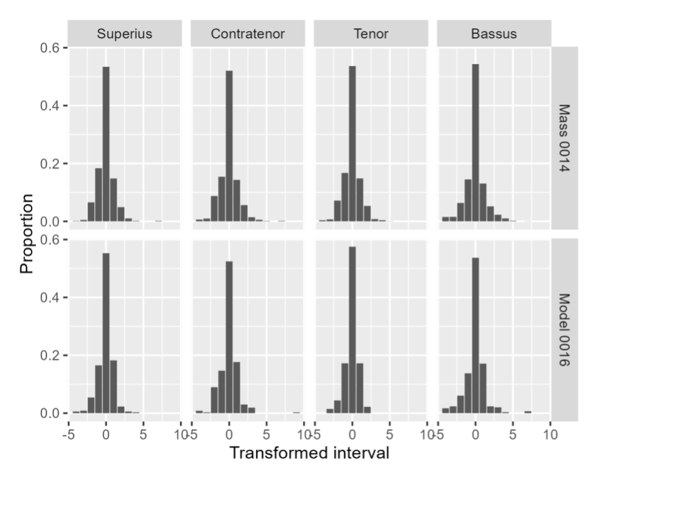
Figure 3: Distribution of interval usage for each voice in Josquin’s Mente Tota and Missa Mente tota. The height of each bar indicates the relative frequency of that interval in the voice line. The height of the bars at 0 reflects that the unison (no pitch change) is the most common interval observed in our sample.

These frequency distributions are a concise way to characterize the overall behavior of a piece. As ever, there is a tradeoff between concision and detail: in this case, we lose all information about where the intervals occur and in what sequence, as with the “bag of words” approach in computational linguistics.

Similarity at Multiple Levels

Single-interval distributions

Given two frequency distributions, as discussed above, we can obtain a mathematical measure of how similar or different they are. There are several statistical tools for this, of which perhaps the most common is the $\chi^2$ statistic. A larger value of this statistic indicates that the two distributions are more different in shape. Figure 4 shows partial results of this analysis on Josquin’s Mente Tota and Missa mente tota. For each voice line (a single voice part throughout a single Mass movement, or the model), we create a frequency distribution of individual intervals, as shown in [figure] above. Then, for each pair of voice lines, we measure whether their distributions are similar. The color of the cell corresponding to a pair of voice lines is lighter if the two lines are different, and darker if they are similar. For simplicity, Figure 4 shows only the results for the Bassus lines. We can see that some specific movements are especially similar or distinct in terms of the interval usage in the Bassus: for example, of all the Mass movements, the Sanctus has a Bassus part most similar to that of the model (as it is the darkest cell in the “Model” row). We can also see that some voice lines tend to be more similar or dissimilar to others overall. For example, the cells in the Gloria row/column tend to be lighter than those in the Sanctus or Kyrie rows/columns; this suggests that the Bassus in the Gloria has a more unusual distribution of intervals (with atypical counts of certain intervals), making it more distinct from other samples, while the Sanctus and Kyrie use more standard distributions of intervals.

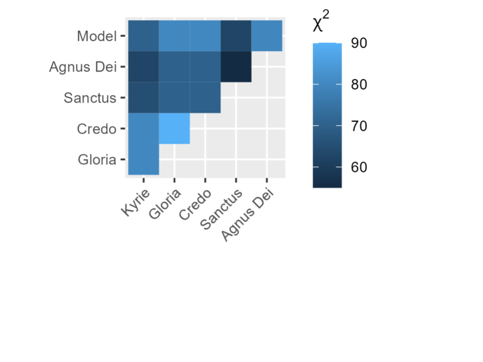
Figure 4. Comparison of the Bassus lines from Mente Tota and each movement of Missa Mente tota. The color of each cell shows the dissimilarity between the two pieces in that row and column, as measured by the $\chi^2$ statistic; lighter shades indicate greater differences.

N-grams, Quotation, and Homogeneity

n-gram distances

When looking at a piece at the n-gram level, we can use methods designed for vectors: sequences of values that have a fixed order, though not necessarily a correspondence to time. There are many measures for the similarity or distance between two vectors. Perhaps the most familiar methods work element-wise, calculating distance between corresponding pairs of values in the two vectors, then combining these to get an overall distance for the vectors. For example, the common Euclidean distance or $L_2$ norm between two vectors $\boldsymbol{a}$ and $\boldsymbol{b}$ has the form $\sqrt{\sum_i (a_i - b_i)^2}$ , while the Manhattan distance uses the absolute value rather than squaring: $\sum_i(|a_i - b_i|)$ .

While the principles of the two measures are similar, Euclidean distance puts greater emphasis on large discrepancies between individual elements, because these differences $(a_i - b_i)$ are squared. Relatively speaking, Euclidean distance will assign a greater distance to two vectors that are mostly similar with a few very different elements, as opposed to two vectors that are slightly different in several elements. For example, according to Euclidean distance the vector (0, 0, 0, 0, 0) is more distant from (0, 0, 0, 0, 2) than it is from (0, 0, 0, 1, 1); while under Manhattan distance both pairs of vectors are the same distance apart. Musically speaking, choosing Euclidean distance indicates that we are particularly interested in cases where two phrases have extreme differences in intervals, if only at a few time points – that such phrases are especially different from each other overall. Choosing Manhattan distance, meanwhile, would reflect the idea that two phrases with several slightly different intervals can be just as distinct. In the examples below, we use Manhattan distance.

Using any chosen distance measure, we can find the distance between any two n-grams, whether in the same piece or different pieces. For example, given an n-gram, we can ask whether that sequence or a similar one occurs in another voice line in the piece: essentially, whether this short piece of melody is reused, or if not, how different it is from the rest of the melodic lines.

In some cases, the n-gram has an exact match, as seen in Figure 5a, which shows the interval representation of the first 250 beats of the Gloria from Févin’s Missa Ave Maria (CRIM Mass 0005). Here, the initial n-gram highlighted in the Contratenor occurs in the Superius voice later in the piece.

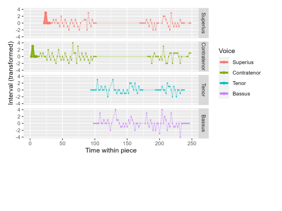
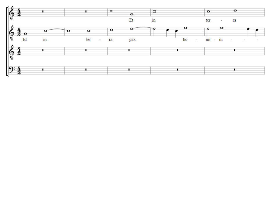
Figures 5a and 5b. Interval representation of the beginning of the Gloria from Févin’s ***Missa Ave Maria*, with a portion of the score. An example** n-gram is highlighted at the beginning of the Contratenor line, as well as an exact match to this n-gram found in a different voice in the same piece. These correspond to the matching entries for each voice seen in the score.

In other cases, there is no exact match to the n-gram; but we can still find the n-gram that is the best match, in the sense of having the smallest distance to the original n-gram. In Figure 6, the highlighted Contratenor n-gram has no exact match elsewhere in the piece; the closest match occurs in the Bassus, just after beat 200.

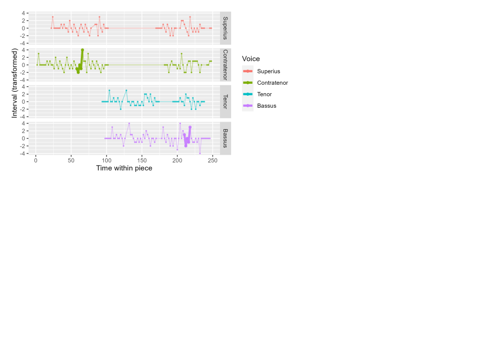
Figure 6. A different n-gram in the Contratenor. This n-gram has no exact match in any other voice in the piece. Instead, we highlight the n-gram that has the lowest distance (greatest similarity), which occurs in the Bassus.

We can calculate this best-match distance for every n-gram in a piece. This creates a new time series with its own potential insights; or, as with individual intervals, we can summarize the values to describe the overall behavior of the piece.

Figure 7 shows these best-match distances for the same selection as discussed above. This representation reflects the development of “distinct” melody in each voice over time. For example, each voice opens with the same phrase, so these opening n-grams all have a best-match distance of 0: they all appear identically in another voice. As each voice line develops, we begin to see n-grams with no exact matches, unique to that voice; this is most extreme in the Bassus (reflecting the tendency for that voice to perform large leaps not seen in other voices), and least prevalent in the Superius (which largely echoes melodic phrases from the Contratenor).

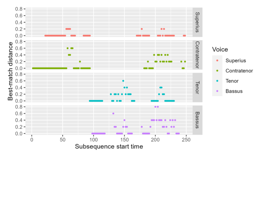
Figure 7. “Best-match distance” representation of the first 250 beats of the Gloria from Févin’s ***Missa Ave Maria*. Each point represents an** n-gram, with the X coordinate showing the start time of that n-gram. The height of the point indicates the distance between the n-gram and its closest neighbor, or most similar match, in another voice in the same piece: n-grams with exact matches have a best-match distance of 0.

Within-piece and cross-piece matching

The discussion above focuses on finding matches for an n-gram within its own piece. In this case the corresponding best-match distances characterize the piece’s homogeneity: when, and how much, it repeats (or nearly repeats) itself. If a piece has a low average best match distance of this type, then most n-grams have identical or near matches elsewhere in the piece: most of the melodic phrases in the piece recur or are echoed elsewhere. If a piece has a high average best-match distance, then it contains many non-repeated melodic phrases—or some phrases that are very different from anything else in the piece (n-grams with a very high distance to their nearest match).

But, because of the particular structure of an Imitation Mass, it is also reasonable to search for matches across pieces. For example, we can calculate the best-match distance of each n-gram in a Mass to that Mass’s model. In this formulation, low best-match distances indicate that the melodic lines of the Mass are largely taken from the model, or are similar to phrases in the model. If the Mass has a high average best-match distance, however, this indicates that more of the melodic content is original rather than quotation. We can then characterize a Mass based on its balance of melodic quotation and original content.

Figure 8 depicts the same selection as above (the beginning of the Gloria of Févin’s Missa Ave Maria); but now we show best-match distances from each n-gram to the model, Josquin’s Ave Maria. This representation allows us to see which parts of the piece use quotation more heavily—for example, the opening n-grams of each voice have best-match distances of 0, indicating that they are exact quotations from the model; the ends of phrases have best-match distances of 0 as well, since the Mass and model use the same types of cadences; but during the melodic development toward the middle of each phrase, there are more n-grams that are very different from anything in the model. In comparison to Figure 7 above, we can also see that the best-match distances tend to be higher when looking across pieces: the Gloria repeats itself (from one voice to another) more closely than it echoes its model.

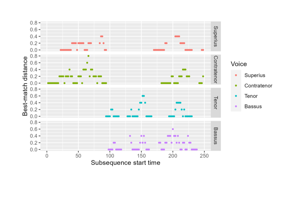
Figure 8. “Best-match distance to model” representation of the beginning of the Gloria from Févin’s ***Missa Ave Maria*. Each point represents an** n-gram, with the X coordinate showing the start time of that n-gram. The height of the point indicates the distance between the n-gram and its closest neighbor, or most similar match, in the model: n-grams with exact matches in the model have a best-match distance of 0.

Summarizing the distances can be particularly interesting here. Figure 9] shows the average best-match distance from Mass n-grams to their corresponding models, separated out by voice (on the X axis). Each line here represents the Kyrie of a different Mass: Missa Ave Maria (CRIM Mass 0005) and Missa Mente tota (CRIM Mass 0014), both by Févin, and Missa Je suis déshéritée (CRIM Mass 0006) by Guyon. In both Févin Masses, the highest best-match distances occur in the third voice (Contratenor), indicating that this voice has the most original development and least quotation from the model. But Guyon’s Mass shows a different profile, with a higher deviation from the model overall, and with the greatest deviation from the model occurring in the first voice (Bassus) and the higher voices staying closer to the model. Thus, using only objective data-driven characterization of the pieces, we have identified a characteristic of Févin’s composition as distinct from Guyon.

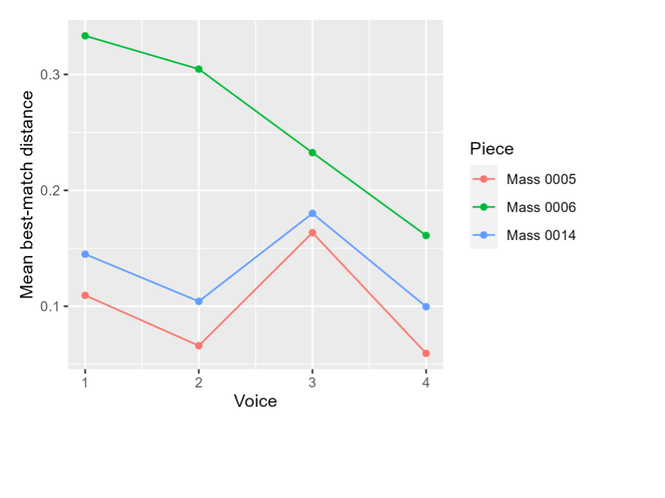
Figure 9. Summarizing best-match distances to the model for each voice line in three different Kyrie movements. Voices are numbered from lowest to highest within each piece (Bassus = 1, Superius = 4). The height of the point indicates the average (mean) best-match distance across all n-grams in that voice line.

Full-piece Time Series Methods

When working with very long n-grams, or the entire time series of a piece or voice, we can draw on statistical methods for time series data—though with care, since typical time series behaviors like trend, seasonality, and autocorrelation may not apply to melodic lines, or may work differently.

One point of interest is the concept of temporal shifting or stretching, as seen in methods like Dynamic Time Warping (DTW). This method is designed to find the similarity (or dissimilarity) between two time series where one series may be shifted earlier or later, or stretched over time. In this case the two time series may be quite different if compared element-wise, time point by time point; but if time $t_i$ for one series is allowed to “stretch” to a different time $t_{i*}$ in the other series, we may find that the series match up more closely. In some implementations, DTW imposes a penalty for stretching times in this way, which is factored into the overall measurement of similarity or distance between the series.

Along with the distance value itself, DTW produces interesting ancillary information: the optimal matching between the time points of the two series being examined, and the cost of possible matches. This can show areas where one time series, or melodic line, is mostly the same as another, or areas where one jumps ahead or stretches out. Figure 10 returns to the example piece from above, showing the opening of the Contratenor line in the Gloria of Févin’s Missa Ave Maria compared against the same voice in its model, Josquin’s Ave Maria. Each voice line’s sequence of intervals is shown in condensed form along one axis; large gaps appear when the voice is resting. The line in the center of the plot shows the ideal matching between time points in the Mass and model, beginning at the start of the piece in the bottom left corner. For example, the matching begins at beat 0 in the Mass and beat 16 in the model, since the Contratenor voice enters later in the model; next we see a diagonal sequence, showing that the best matching pattern is to proceed forward through both voice lines (reflecting the fact that the opening melody is the same in both). The coloring in the plot overall reflects the cumulative cost of matching a given time point from the Mass (X axis) to a given time point in the model (Y axis), with light (yellow) colors corresponding to higher cost and dark (blue) colors to lower cost. Shifting many time points incurs a large penalty—hence the very high cost in the bottom right corner— but we can see that there are small diagonal “streaks” or areas of relatively low cost throughout the plot. These indicate sequences or phrases that could be effectively matched to phrases occurring in the other piece at different times.

The standard DTW implementation shown here has a number of shortcomings for this application. For one, it treats time as monotonic, or one-directional: the algorithm looks for a match for each interval in the Mass in sequential order, given the matching it has already done, and it is not possible to “stretch backward” or re-match time points to an earlier part of the sequence in the model. Monotonic time is generally a reasonable assumption, but inappropriate to a musical context, where one melodic line may quote disparate parts from another, or return to echo an earlier musical phrase. This implementation also takes a fairly simple approach to local distance, simply attempting to find an exact match to each interval within an allowable time window; but in practice, we may want to allow inexact matches (or non-matches) in the interest of better alignment overall, or seek to emphasize certain matches over others. Extending the method to find these disparate matching possibilities, while still using penalized stretching at a local level, is an intriguing possibility for future analysis.

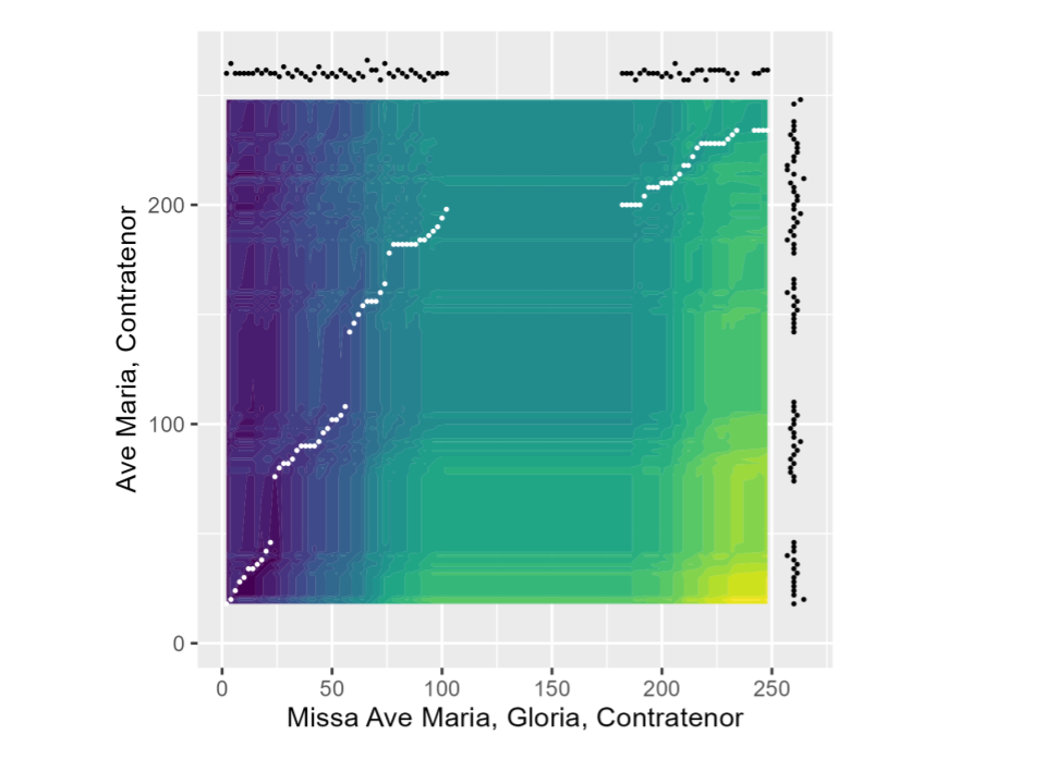
Figure 10. DTW cost representation of two voice lines from separate pieces. The Contratenor line from the Gloria of Missa Ave Maria proceeds along the X axis, while the Contratenor line from the model proceeds along the Y axis from bottom to top. The sequences of intervals in each individual voice line are shown in the margins of the plot. The sequence of white dots moving through the plot shows the best matching pattern between the two voice lines as found by the algorithm, while the color of the background indicates the cumulative cost of matching each time point from the Mass (X coordinate) to a time point from the model (Y coordinate).

Conclusions and Future Work

We have given a brief survey of methods for measuring similarity between melodic objects, whether short phrases or entire pieces, but there are many ways to adapt and expand these techniques in future. The choice of distance and similarity measures—whether one of the conventional metrics or a new measure specifically adapted to the musical context—can affect the results and help the analysis focus on different musical characteristics. These ideas can also be extended beyond a single melodic line, by including stacked intervals that reflect the harmonic distance between simultaneous pitches, duration information, and so on.

Beyond simply measuring the similarity and distance between two objects, we can use these similarities to group objects together. Supervised classification algorithms can be used to assign objects to known groups, while clustering can find groups of similar objects without any previous training. For example, by applying similarity methods to all pieces in the CRIM corpus, we may be able to characterize specific composers, regions, or time periods; or we may be able to find groups of kindred compositions that reflect a different type of shared behavior. Exploring variations and extensions of the methods described above, and using them for comparison and classification, will provide a wide range of opportunities for future work.

References

Giorgino T (2009). “Computing and Visualizing Dynamic Time Warping Alignments in R: The dtw Package.” Journal of Statistical Software, 31(7), 1–24. doi:10.18637/jss.v031.i07.

R Core Team (2021). R: A language and environment for statistical computing. R Foundation for Statistical Computing, Vienna, Austria. URL https://www.R-project.org/.

Tormene P, Giorgino T, Quaglini S, Stefanelli M (2008). “Matching Incomplete Time Series with Dynamic Time Warping: An Algorithm and an Application to Post-Stroke Rehabilitation.” Artificial Intelligence in Medicine, 45(1), 11–34. doi:10.1016/j.artmed.2008.11.007.
Wickham H, Averick M, Bryan J, Chang W, McGowan LD, François R, Grolemund G, Hayes A, Henry L, Hester J, Kuhn M, Pedersen TL, Miller E, Bache SM, Müller K, Ooms J, Robinson D, Seidel DP, Spinu V, Takahashi K, Vaughan D, Wilke C, Woo K, Yutani H (2019). “Welcome to the tidyverse.” Journal of Open Source Software, 4(43), 1686. doi:10.21105/joss.01686.